A few weeks ago I attended the first edition of what turned out to be a great event, RTC.On, and I took that opportunity to submit a talk on something I wanted to work on for quite some time: bandwidth estimation in WebRTC and, more specifically, Janus. The main objective of that presentation was not only to “force” myself to work on this topic and share the results, but also to try and provide everyone with some more insight on what is ostensibly one of WebRTC’s best kept “secrets”: not out of malice (at least I don’t think so), but because of how complex and obscure it actually is when you start digging into it.
While you can watch the video of that presentation here, and check the slides on Slideshare, I thought I’d also write down a blog post to talk about that effort: where we are and, most importantly, what’s still missing. I know there’s many people trying to address similar challenges, so in case anything you’ll read here resonates with you, please do get in touch and let me know!
What do you mean by “bandwidth estimation”?
This is indeed a tricky one to answer, as most people (me included) often conflate in that term multiple different things that don’t strictly belong to that, like congestion control for instance.
In a nutshell, bandwidth estimation (or BWE in short) is, well, whatever can be attempted to figure out how much data you can send on a connection: within the context of WebRTC, how much data per unit of time (e.g., seconds) you can send to your peer over a PeerConnection. It’s clear that this is quite an important piece of information to have, since in a WebRTC session you’ll most definitely not want to:
- send more than you can (your own network limitations);
- send more than the network can accommodate (the media path between you and the peer may have some bottlenecks);
- send more than your peer can actually handle (network or processing limitations on the receiver side).
Again, there’s some confusion here sometimes, where many confuse the process of figuring how much you can send, with actually acting on it to avoid congestion: the latter is usually called, aptly so, “congestion control” (CC), and involves the actual attempts to avoiding and handling network congestion in the first place. Just as I did in the presentation, for the sake of simplicity I’ll indeed conflate the two concepts when talking about BWE: just know there are more things happening besides just “estimating”!
At this point, you may be wondering: what’s so special about WebRTC and BWE/CC? After all, something like that happens all the time already when, for instance, we download a file over the Internet, or browse to a website. The main difference, obviously, is that the latter are all examples of delivery of data over reliable connections, e.g., via TCP: depending on the network constraints that may be present anywhere on the path between sender and receiver, CC may kick in to, e.g., slow down or speed up the delivery of data, typically depending on a congestion window. As a result, delivery of the same amount of data may take more, or less, time: eventually, all bytes will be transferred. A super ugly visual representation is the following.

As you may have guessed, this is not a luxury we have in WebRTC. In fact, unlike the examples we’ve made just now, in WebRTC all streams are actually real-time: this means that slowing down the delivery and have data be delivered, e.g., in a few seconds rather than right away, is not an option at all. The way a WebRTC session is supposed to react to constraints of that sort is to somehow “adapt” the data itself, so that the same (or most of the) information can still be delivered as quickly as possible, without skipping a bit and trying to fit in what’s available. That’s why having a prompt and, where possible, accurate overview of what the available bandwidth is becomes of paramount important: once a WebRTC sender knows what the available bandwidth is, it can, for instance, try to reconfigure the audio and video encoders so that the data being pushed on the network stays within those limits (e.g., by reducing the video resolution and the bitrate). This is how WebRTC actually works in the wild today (we’ll explain a bit more in detail how in a later section), and why whenever you do a peer-to-peer WebRTC session you may see the quality of the streams you get from the peer change in real-time, while still remain up and running despite challenging networks.

Of course, not all WebRTC senders can actually react the same way. While a browser, for instance, can indeed react by dynamically changing how the encoder works, that’s not what a server like an SFU (Selective Forwarding Unit) can do instead. In fact, SFUs just relay media coming from other participants, which means they don’t actually have access to the encoder itself: they’d have to react differently.
They could, in principle, just forward any estimation they receive from subscribers of a specific stream to the participant that’s originating the stream itself, so that they can in turn reconfigure the encoders accordingly, but that would actually work poorly: the participant could be flooded with confusing feedback, if done wrong; but even done right, e.g., by only forwarding the “worst” feedback received, the result would still be a bit of a mess, since it would make the media source adapt to the weakest subscriber link. Even a single participant on a “crappy” network would end up “ruining” the experience for everyone else, since the encoder would be updated to accommodate the network requirements of that impacted participant.
Luckily enough, that’s where WebRTC features like simulcast and SVC can be of a great help. We’ve talked about both a lot in previous posts (like here and here, for instance), so I encourage you to go read those if you’re still unfamiliar with those terms, but in a nutshell they both envision ways for a media publisher to contribute multiple “options” for the same stream (e.g., the same video stream at different resolutions, and so different bitrates), allowing subscribers to choose the best one for their current requirements (whether it’s network limitations, or current application requirements). From a visual perspective, it looks a bit like this, where different subscribers may actually receive different versions of the same contribution.

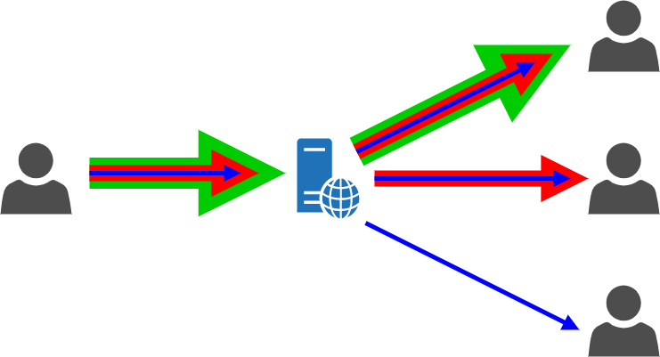
The main difference between simulcast and SVC is that the former works by encoding different video streams as separate/parallel streams at the same time, while SVC encodes multiple streams into one using some sort of “onion” layering (don’t quote me on that!). For the purpose of this blog post, the distinction is actually not that relevant: what’s important is that, in both cases, the SFU has access to different streams from the same media publisher, thus being presented with a way to somehow send “less” or “more” data depending on what a subscriber actually can receive.
Using a similar graph as the one we presented before, it means that, for the WebRTC scenario, we can imagine BWE/CC working a bit like this, where HQ/MQ/LQ stand for High Quality, Medium Quality and Low Quality (thus representing the different options simulcast or SVC may be offering).

The graph suggests we can adapt to a more narrow network path on the way to the receiver by just switching to a lower quality version of the stream (which will of course also have a lower bitrate, and so less network requirements). As we’ll see later on, it is a bit more complicated than that, but that already gives us an important piece of information, especially when thinking of how to get something like this to work in a server like Janus (e.g., in the VideoRoom SFU plugin).
That’s great! How do we do it?
That’s the million dollar question, isn’t it? 
In general, congestion avoidance in real-time session is a tricky pickle. A few years ago, the IETF formed a Working Group specifically devoted to solve that exact issue, called RMCAT (RTP Media Congestion Avoidance Techniques). The work of that WG is now concluded, and several different options were discussed, most importantly:
- SCReAM (Self-Clocked Rate Adaptation for Multimedia);
- NADA (Network-Assisted Dynamic Adaptation);
- and GCC (Google Congestion Control).
While SCReAM and NADA both became RFCs out of the WG efforts, GCC remained just a draft. That said, when you look at what’s actually available in the wild, you’ll notice that GCC is, as a matter of fact, the only option that’s widely deployed. In fact, it’s what libwebrtc uses, which makes it what the overwhelmingly vast majority of WebRTC endpoints use as well.
In a nutshell, GCC works by implementing a combined usage of an RTP extension and dedicated RTCP feedback, using a mechanism called TWCC (Transport-wide Congestion Control). To keep it simple:
- the media sender implements a global and monotonically increasing sequence number across all media streams;
- for every outgoing RTP packet, the media sender adds an RTP extension that contains this sequence number (again, monotonically increasing as each RTP packet is sent);
- media receivers that get those RTP packets extract this global sequence number piece of information, and then use them to address those packets in specifically crafted RTCP feedback messages;
- the media sender processes these RTCP feedback messages, and uses them to estimate the bandwidth and then react accordingly (e.g., adapting the encoder bitrate).
If this sounds like magic, well, a bit it might be, but there’s a specific logic behind it that we’ll cover later, especially in how that feedback is crafted, what info it contains, and how that info can be used. What’s important to understand at this point is that this is a sender-side bandwidth estimation: the sender adds some addressing info to packets, the receiver gives their view of how the packets got there, and the sender can use this perspective to figure out if there are problems in the network that might need a change in their current estimate of the available bandwidth.
Now, this is all wonderful, but the main question is: GCC works great for endpoints with access to an encoder (we’ve explained how it’s what libwebrtc uses, so you’re actually using it any time you join a WebRTC session), but can it help when trying to implement BWE in a server as well, as we’ve discussed before? Or should we look at something else?
So many options!
To answer that big question, I first of all tried to learn a bit more about GCC, but that’s when I encountered the first big obstacle… the main information about it come from the aforementioned draft and a paper from the authors, but both are now apparently very outdated! While they may have provided a very detailed overview on how GCC worked early on, the implementation in libwebrtc evolved a lot, and is apparently now very different from what’s documented, making any effort to study it quite problematic (and I was most definitely NOT going to reverse engineer the libwebrtc code to figure that out).
The second big obstacle was that, even in the existing documentation, most of the information about how the algorithm worked were quite complex, and probably made me look a bit like this famous meme.

This prompted me to start looking into NADA instead, but that seemed pretty complex as well. Besides, while just as TWCC it relies on RTCP feedback to work, it uses a custom RTCP feedback format specified in RFC 8888, which unfortunately no existing WebRTC implementations support (we’ve explained how libwebrtc uses GCC/TWCC exclusively). While there have been efforts to prototype NADA in custom Firefox builds by having it rely on the existing TWCC RTCP format, to my knowledge there’s not much information available on that, and besides it looks like the kind of feedback TWCC provides is only a subset of what NADA typically expects from the RFC 8888 feedback, which makes me think it would probably work in a suboptimal way as a consequence.
That led me to some conversations with other WebRTC experts on the topic, to try and figure out what most end up doing and how. In fact, as I anticipated initially, BWE is a quite obscure topic when you start investigating it: very little information beyond the most high level concepts can typically be found, and when you try digging a bit deeper, there’s not much to be found. You’ll find many people asking about it on different forums, with not that many (useful) responses. That’s why I called it one of WebRTC’s best kept “secret”: I don’t know if it’s because it’s too complex to explain, or because those that know about it prefer to keep it a mystery to better profit from their knowledge. I tend to think it’s more of the former, rather than the latter, since the WebRTC community I’ve engaged with so far has always been very cooperative.
Those conversations mostly highlighted an important point: while some did implement their own version of GCC, many don’t seem to see it as a good fit on the server side, and ended up implementing something different (e.g., like Sergio did in Medooze). That eventually convinced me to take that road too, and try to figure out what staples to start from in order to build something simpler from scratch: something that would probably not perform as well as established algorithms, but at the same time something I’d be more familiar and comfortable with, making tuning and updates much more manageable in the longer term as well.
Building BWE from the grounds up
In order to build something from scratch, I knew I’d first need to figure out which building blocks to use, that is, what foundations would be needed in order to get it work in the first place. The time I spent studying GCC helped me understand some of the core concepts most algorithms use, that I decided would be the ones my own algorithm would be based upon as well. Namely, the main staples of a real-time BWE can be considered the following:
- acknowledged rate (that is, a rough estimate of the bandwidth out of the packets we know the receiver got, from their feedback);
- a loss based controlled (that is, how to react to packet losses);
- a delay controller (that is, how you can try and predict congestion by looking at interarrival delays);
- packet probing (that is, what you use to try and test when you can send more than you’re sending now).
All those bits are actually quite important, even though for different reasons, and as we’ll see some are a bit more important than the others. In order to better understand why they matter, and how they can actually help estimate the bandwidth and do something about it, let’s try and go through each one of them.
Acknowledged rate
When introducing TWCC before, we’ve explained how it combines the usage of an RTP extension (to RTP packets) and a custom RTCP feedback (to provide feedback on those packets). One of the pieces of the information this RTCP feedback can provide is indeed which RTP packets the receiver actually got, since they’re all indexed by the global sequence number available in the RTP extension.
This very simple assumption already helps us understand something quite important: if we keep track of how “large” each RTP packet we sent was, by knowing which packets the receiver got we can already obtain a first very rough estimate of how many bytes actually got through of those we sent in a specific time frame. This is indeed what the “acknowledged rate” is, and as you can guess it’s already a very useful piece of information, since it can give us some sort of “lower bound” for the BWE: if just now these bytes made it through, then we have at least that much available bandwidth.
Of course, as an estimate it’s a very rough one, at best… in fact, first of all it’s bound to what we’re currently sending, which may not be much, or not enough if we’re interested in sending more. That said, what the acknowledged rate tells us is that, for sure, this data did make it through, and so we have a foundation for our BWE. This makes it a precious piece of information, since it means it’s something we can start from (as soon as we begin a new session, for instance), and also something we can fall back too when we encounter some problems (e.g., we detected congestion sending Y, but since X<Y was our acknowledged rate, let’s assume our estimate is now X).
But, again, on its own it’s not enough for obtaining an actual BWE. We’ll need other things to work in conjunction with it too, especially if we want to figure out when we’re hitting a bottleneck, or when we can actually try and send more than we’re doing now.
Loss based controller
To figure out if something’s going wrong, looking at packet losses does seem like the obvious thing. In fact, if the recipient is telling us they didn’t receive some packets from us, then it may be an indication that something, including congestion, may be causing these problems. As such, a kneejerk reaction may be to slow down immediately when losses are reported, and decrease the current bandwidth estimate as well.
In practice, it’s not that simple, and this comes with a few drawbacks. First of all, using losses is, by definition, a “reactive” mechanism: we’re reacting to something that happened already (packets were lost on the network), which means anything we can do can only happen after this something took place. As a result, things like video freezes or artifacts may have happened already.
What’s also important to understand, though, is that it can’t be given for granted that the presence of losses is actually related to network congestion. When using non-wired connectivity, losses may occur for a wide variety of reasons, and may actually be sistemic even in presence of a very good connection. This means it’s equally important not to overreact to packet losses, as they may very well be occasional, or again part of the nature of the physical layer.
What algorithms like GCC do is implement some thresholds for packet losses, implementing different reactions to different levels of losses. The draft, for instance, does something like this:
- if losses are less than 2%, then assume everything’s right, and keep increasing the estimate;
- if losses are between 2% and 10%, then keep the estimate where it is;
- if losses are higher than 10%, then assume something’s wrong and decrease the estimate.
As you can see, those percentages are sensibly higher than the thresholds one could intuitively come up with, thus again suggesting that, although losses play an important role in figuring out there’s an issue, at the same time they shouldn’t be overestimated.
When it comes to how a sender can be aware of losses in the first place, there’s actually many different ways of doing that. There definitely are the standard RR (Receiver Report) RTCP messages, for instance, but the TWCC RTCP feedback message can also be used for the purpose, since as we’ve seen in the previous section talking about the acknowledged rate, it does contain info on which packets have been received and which haven’t (yet?).
Delay based controller
While a much less intuitive concept to grasp, delays have become one of the most important indicators of possible congestion. They’re at the basis, for instance, of algorithms like BBR, which have become much more widespread lately for congestion avoidance purposes.
The main idea behind it is the concept of bufferbloat, that is the fact that, as packets traverse the network, they will end up being handled by different buffers along the way. In the presence of congestion, packets may be kept in these buffers for a while longer, until they’re ok to be sent, which means a delay will be introduced as a consequence: this delay may grow in case the congestion persists or grows worse, as more packets could be kept in the queue. As a consequence, in the presence of congestion a media receiver could receive packets with higher interarrival delays then the delays at which those packets were actually sent from. The following graph, taken from Mathis Engelbart’s excellent presentation on how he added BWE to Pion, helps understanding this from a more visual perspective.

This suggests that analyzing these interarrival delay patterns could actually help detect congestion before it occurs, or at the very least early enough in the process to do something about it. This makes a delay based controller much more proactive than the loss based controller we introduced before could ever be, since it might allow us to adapt to, and possily avoid, congestion in the first place.
Of course, in order for this to work it means two things must happen:
- the media sender must keep track of when it sent each RTP packet (to know the relative inter-send delays at which they were sent over the network);
- the media receiver must analyze the interarrival delays of the RTP packets it receive, and provide feedback back to the sender.
This is exactly what the TWCC RTCP feedback was meant for. Besides providing information on whether a packet was received or not, in fact, it will also be used to specify, for each RTP packet (indexed via the global sequence number received in the extension) the level of delay from the previous one, thus providing the sender with this precious information.
At this point, the sender can use the interarrival delays information to try and figure out if congestion is occurring, or about to occur. How to do that is indeed part of the “magic recipe” of BWE, since again it’s not important to overreact to what could be, e.g., occasional delay fluctuations, rather than actual bufferbloat occurring somewhere in the network. Again, this graph from the BBR documentation provides some helpful insight.

It explains, for instance, the difference in how delay- and loss-based controllers operate: besides, it shows the optimum operating point, but considering feedback from the receiver is involved (which does involve some round-trip times), where the algorithm actually operates is a bit further along the road, but still much sooner than losses detection would allow to.
Probing
All we’ve seen so far covers “where we are” and “is something wrong?”, and so can help handling lowering the estimate in case of issues, or staying there if all is good. A good chunk of BWE is also in trying to figure out when we can actually send more, though, and so in when we can try increasing our BWE estimate as a consequence. This is particularly important, for instance, if due to network issues some time ago we’re now receiving a lower quality of a video stream, but we’re still interested in receiving a higher quality stream when possible. We can’t figure that out using just the tools we’ve gone through so far, though: the acknowledged rate won’t help, for instance, because it will just tell us that the lower quality stream is going great (all packets were received); losses and delays won’t help either, since again the only thing they can tell us is that there’s no congestion sending what we’re sending now.
In a regular endpoint the WebRTC sender might slowly increase the encoder bitrate when things go well, and then stop as soon as there’s a bump in the road (e.g., congestion is increasing). As we’ve already established, though, WebRTC servers, and SFUs in particular, are not “common” endpoints, especially considering they don’t have the flexibility to just tweak some encoder settings to modify the outgoing data: they need to work with the streams that are coming in. Simulcast and SVC layers can help, since they give us different bitrate levels we can jump to or from, but in most cases their bitrate patterns will be distant enough that we often can’t just go from one to the other indiscriminately: we’ll need to somehow and more seamlessly ease into one.
This is where bandwidth probing can actually help. In a nutshell, probing is the process of injecting “artificial” packets along the regular one (actual RTP packets being sent) for the sole purpose of adding some bits to the traffic. If these artificial traffic are handled the same way as the regular streams are (e.g., RTP extension plus RTCP feeback addressing them), this means that the additional traffic does count for the purpose of figuring out our estimate. If nothing wrong happened by adding this artificial traffic (there was no congestion) it means our estimate can be higher than before; if we do this enough times and long enough, ideally it will get us to a point where we can figure out we have enough bandwidth for, e.g., a higher simulcast or SVC layer. Once there, if there’s even higher qualities we can aim for, we can do it once more, starting from the acknowledged rate we now have. A simple visual representation of this process is provided in the graph below, which shows probing being added to switch to a different target.

Again, how to actually implement probing is another of those WebRTC mysteries, since there’s different approaches when it comes to what to use as artificial traffic, how much to send of it, how often, etc. Considering that these probing packets must be handled the same way as regular RTP packets are, it means they need to be RTP packets themselves: some choose to generate new RTP packets made of just padding for the purpose (that the receiver would automatically discard, as a consequence), while others prefer to use retransmitted packets for the job (rtx). We’ll see shortly how I ended up implementing them myself.
Let’s get some BWE in Janus, shall we?
Now that we’ve gone through the different foundation we needed for implementing a new BWE algorithm, we can see how they were put all together to work for a first integration in Janus itself. As anticipated, the main objctive was figuring out a good BWE mechanism for Janus to use, for a specific purpose: allowing Janus (and its plugins) to have an idea of how much media recipients can receive at any given time, and where possible try to adapt accordingly.
The first challenge came from the nature of Janus itself. In fact, unlike most WebRTC servers out there, Janus is a general purpose one with a modular architecture. It has a core that is responsible of all the WebRTC aspects (e.g., ICE, DTLS, SRTP, RTCP termination, data channel management, etc.), while negotiation and what to do with the media is left up to application/media plugins instead. This allows Janus to wear different masks for different WebRTC PeerConnections, e.g., implementing SFUs, audio mixer, SIP/RTSP gateways and so on and so forth.
This allows for a very flexible management of media streams, but it also means that any BWE integration needs to be somehow “hybrid” in nature. In fact, we’ve seen how BWE is made of different bits and pieces that need to work together, and not all of them can be taken care of by the WebRTC core itself in Janus. More specifically, the core can definitely take care of TWCC, monitoring losses and delays, performing probing, and most importantly generating a BWE estimate, but what it cannot do is actually act upon the generated estimate: in fact, as anticipated it’s plugins that decide what to do with the media, which also means it’s plugins that know the relationships between different WebRTC legs (e.g., who’s a publisher, and who’s subscribed to that publisher). As a consequence, it’s indeed up to plugins to somehow make use of whatever BWE estimate the Janus core comes up with: for instance, to decide when to perform a simulcast layer change for a subscriber, or what the next bitrate target will be (e.g., for probing purposes). Most importantly, it’s also up to plugins to decide when to perform BWE in the first place: in this first integration, it’s always disabled by default, and plugins can decide when it’s actually worth it to take advantage of it (it may make less sense if simulcast is not involved, for instance).

All of this was implemented in an experimental PR, that is already in a usable state. As such, if you’re interested in giving this a try, please refer to that link to checkout the related branch.
Let’s have a look at how the integration was performed a bit more in detail, specifically related to the four staples we mentioned in the previous section.
Janus core BWE integration
As anticipated, although plugins are involved in the process, the Janus core still takes the lion’s share of activities that are required for BWE. It is responsible, for instance, of generating the RTP extension with the global sequence number, processing TWCC feedback from recipients, monitoring losses and delays out of the feedback it receives, performing probing and so on, up to the actual generation of a BWE estimate that plugins can use.
In order to do that, we added a new object to the core, a BWE context, that is continuously updated over the lifecycle of a PeerConnection once it’s created. More specifically:
- Any time an RTP packet is sent over the PeerConnection, the global sequence number RTP extension is added to it, and the core keep tracks of some information related to the packet itself (the sequence number it was assigned, how large the packet was, when it was sent and the delay from the previously sent packet), including information on the nature of the packet itself for statistical purposes (e.g., whether it’s a regular RTP packet, a retransmission, or probing we’re generating). All this info is saved in this new BWE context.
- The context is also updated any time TWCC feedback is received from the recipient, as it allows the context to keep track of the acknowledged rate (since we saved info on each sent packet), losses and interarrival delays. Any time feedback is received, a new estimate is also computed, using the info that was accumulated over time, thus ideally proving an estimate that is more accurate as more feedback pours in. This is also when the core decides congestion is taking place, for instance, to perform internal context state changes (which could affect the way probing is performed).
PeerConnections in Janus are loop-based, meaning there’s an event loop that runs all the time to keep it updated, and possibly perform actions on a regular basis. When a BWE context is created, a new source is added to this event loop, which is used to dynamically react to some triggers coming from plugins (e.g., when to enable or disable BWE). It’s also used to physically perform some activities, like preparing and sending probing packets, when needed (using pacing to distribute outgoing packets more or less evenly), and notifying plugins about the current BWE estimates under certain conditions. More precisely, at the time of writing plugins are notified about a new estimate either on a regular basis (every 250ms, by default), or whenever the status changes to either lossy or congested (since we’ll want to be able to react quickly).
In a nutshell, this is all the core is supposed to do. It may not seem like much, but don’t forget that computing the current estimate is part of these activities, and that’s where most of the complexity resides. In fact, we’ve discussed how figuring the right thresholds for the loss and delays controller is quite important, just as figuring out how much to probe. In my experience working on this effort, I’ve indeed spent most of my time tweaking the different parameters related to when to trigger some specific conditions, in order to try and figure out how to detect congestion properly, and early enough to be able to anticipate it. We’ll spend some words on this later on, when I’ll show some limited data related to the tests I made.
The simplified diagram below summarizes the core behaviour when processing an incoming TWCC message, and how that can result in status changes and calculations of a new estimate.

As you can see, it’s a relatively straightforward process, where most of the logic sits indeed in ensuring the different parameters are tweaked and tuned appropriately (which is why testing is quite important). As a matter of fact, I don’t see the logic above as cast in stone, and I expect this to change in some parts as experimentation goes forward.
Integrating BWE in the VideoRoom
Once the BWE context was added to the core, it was a matter of adding the missing bits to plugins as well, or at the very least one plugin to start with, in order to make some tests. I usually use the EchoTest plugin when I want to prototype new functionality in Janus, but considering BWE makes the most sense when used in an SFU kind of scenario, I decided to use the VideoRoom plugin as a testbed instead, since it would allow me to separate BWE related to publishers (which we had already) from BWE related to subscribers (the objective of this effort).
Considering the prototype nature of this effort, I decided to keep it relatively simple in this first integration. Specifically, I tied the BWE activities to simulcast only (no SVC yet), and assuming WebRTC subscriptions containing a single video stream (so that I could see more easily the impact of BWE estimates on simulcast layer changes).
As anticipated, in the Janus BWE integration plugins take the role of “enforcers”, meaning it’s up to them to actually do something with BWE estimates. In fact, the Janus core can generate all the estimates it wants, but if no one does something with them, then there will be no actual benefits as far as the user experience is concerned. This means that, for the purpose of this integration, the VideoRoom plugin had some new responsibilities:
- First of all, deciding when to enable BWE for a new PeerConnection: in this case, I decided to only tll the core to enable it for subscriptions involving a simulcast stream.
- Tracking the bitrates of simulcast publisher streams over time: if we want to know when we can switch layer depending on a new BWE estimate, in fact, we obviously need to know what the bitrate of the target simulcast layer is, before we can decide the estimate is enough to support it.
- Keeping track of what the next simulcast layer a subscriber is interested in, and notify the core about it by specifying its bitrate as the target to “chase”: in fact, as we mentioned the only way to know if we can send more than we’re sending now (e.g., the middle layer of a simulcast stream) is probing, but the only way the core can figure out how much to probe is if the plugin tells it what the target is (e.g., the high simulcast layer), so that the core can generate enough traffic to slowly fill the gap and check if no congestion occurs.
- Finally, using the BWE estimate as notified by the core by deciding what to do: e.g., drop to a lower simulcast layer if the current estimate says there’s not enough bandwidth for the current layer, or switching to a higher layer once the estimate tells us there’s enough bandwidth to make the jump.
As you can see, even though the plugin’s responsibilities are apparently less complex than the core ones, they’re still comprehensive enough to ensure they’re done properly. The decision process itself is particularly delicate, for instance: in fact, deciding when to go up or down the simulcast streams can easily cause more harm than good, if these changes occur very frequently, e.g., because the estimate dances dangerously along the line that separates one layer from the other. Being conservative about changes and implementing some cooldown periods can help greatly in that regard, even though being too conservative about them could also slow down ramping up when things are fine again.
Just as I did with the core, I spent a lot of time trying to fine tune and tweak the settings of the code, and there’s definitely more improvements that could be done.
Experimenting with BWE
As soon as a first integration became available in both core and VideoRoom, I started making some tests and experiments, which of course helped greatly with the tweaking to the different parameters related to BWE. I explained how I made a few assumptions with respect to the VideoRoom integration, which means I simplified my BWE testbed as well, by basically having a single publisher available in a room (a publisher with an audio and a simulcast video stream), and a single WebRTC subscription to that publisher aiming for the highest quality possible.
Having publisher and subscriber in separate PeerConnections allowed me to implement network constraints in a much finer grain: specifically, leaving the publisher untouched (so that all simulcast layers would always be available at any given time) while applying dynamic limitations to the subscriber PeerConnection instead. In order to simulate network constraints on the subscriber, I made use of an open source tool called comcast, which is basically a high level wrapper of the well known tc and iptables Linux applications. A simple example is the following:
comcast -device lo -target-addr 1.2.3.4 -target-port 20346 -target-proto udp -target-bw 700The example above instruct tc and iptables to limit the bitrate going to the 1.2.3.4:20346 UDP address (e.g., the recipient RTP address) to 700kbps. As a result, any attempt to send more data than that to that address will result in buffers starting to queue packets. This was exactly what I needed to simulate bottlenecks in a specific WebRTC PeerConnection, and check whether the new BWE code would react accordingly.
Rather than just observe the result visually (e.g., checking whether simulcast layers would be changed accordingly), I was of course also interested in monitoring more closely how the algorithm performed in different circumstances. In order to do that, I borrowed some concepts from Sergio’s stats viewer, and so updated the Janus code so that it could generate different stats related to the BWE operations. Specifically, I configured it so that stats could either be saved to a CSV file (for offline processing), or pushed as live stats to a UDP backend (for live monitoring). In order to visualize those stats (offline or online), I created a very simple Node.js application leveraging Chart.js. While at the time I made the presentation this tool wasn’t publicly available, I decided to release it as open software too, so that more people could use it for debugging: you can find it in the meetecho/janus-bwe-viewer repo.
An example of data is visualized is presented in the two graphs that follow.
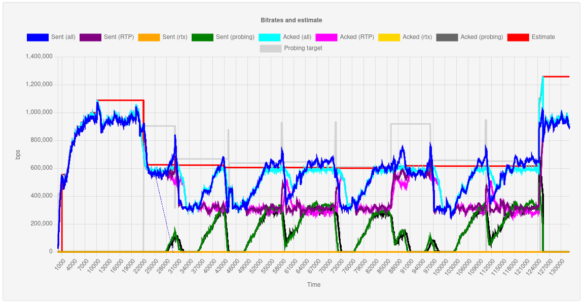

The two graphs represent two different time series for the same time base. Specifically, the first graph depicts different bitrate values, namely the outgoing bitrate of different categories of packets (regular RTP, rtx, probing), the acknowledged rate of each of them, the probing target and the BWE estimate the core came up with. The second graph, instead, is a visual representation of delay-related information, specifically a few different average delays, including the one we weighted to detect trends, and the BWE status (where, for instance, 3 equals to congestion, 4 to recovering, and 1 to all-good). You can refer to the BWE viewer repo for a meaning of the individual properties that are available in the stats.
As you can see from the graphs, all was fine at the beginning, leading Janus to estimate about 1.1mbps of bandwidth up to a certain point. After about 22 seconds, congestion was detected (it’s when I had started the comcast tool to limit the bandwidth to 700kbps). This led the plugin to drop to a lower simulcast layer, one that sent about 600kbps, and inform the core about the new probing target (the layer where we were before). After a few seconds, the core start slowly probing, but this causes traffic to exceed the available bandwidth, thus causing congestion again, and causing a new simulcast layer drop to one that weighs about 300kbps: as a result, the probing target is updated again to a lower value than before (since now our immediate target is not the highest quality anymore, but one a few steps below). Looking at the graphs you can see how the core tries to continuously probe to go up again, using some build-up to get there; this sometimes succeeds in getting us to a higher layer, but since this layer is very close to the available bandwidth threshold, that state is more unstable, thus sometimes causing a congestion again that brings us back to where we were before. Eventually, at about 120s the comcast constraints are lifted: probing manages to stay there for longer, and finally allows to escalate to a higher layer without congestion bringing us down again. We successfully went back to the highest quality we went for!
As such, as you can see the BWE estimate was more or less precise the whole time: when we enforced a 700kbps limit, the BWE estimate stayed around 600kbs, which makes sense, since TWCC was only keeping track of video, and there was untracked traffic contributing to the mix (audio, RTCP, signalling), thus leaving us less headroom. The relative instability in the middle was mostly caused by our occasional attempts to try and see if we could go back up, via probing: probing would hit a wall, and we’d go back to where we started, until constraints were lifted and probing got us back to where we actually wanted to be.
From a user experience perspective, my tests were fine but could be better. The relative instability I mentioned, for instance, could sometimes cause some quick simulcast layer changes, and as a consequence an occasional freeze that would be fixed shortly after that by a keyframe. Getting this process to be smoother is indeed part of all the tweaking I’ve tried to do on the different parameters, from delay detection thresholds to probing ramp-up. Tweaking those parameters is something that you can easily end up doing forever: being more conservative, for instance, may make the “unstable” phase smoother, but would also considerably slow down the ramp-up when constrains are lifted; being more aggressive makes ramp-up when things are fine great, but can also potentially lead to more layer changes than the current situation warrants, thus contributing to the instability period.
This definitely is an ongoing effort, but as a prototype I was very happy about the result! As confirmed by the graph above, BWE was indeed doing its job, which is not something I gave for granted, especially considering it was built from scratch starting from some basic concepts.
What’s next?
Apart from more tweaking, there’s actually a lot that still needs to be done. More testing is definitely key, here: in fact, local tests with the help of tools like comcast help, but are not always representative of real scenarios that can lead to trouble. This is one of the areas where I hope the Janus community will help: having the BWE PR and the stats viewer application available should make it quite easy for insterested people to tinker with it and see what they get out of it.
You may also have noticed I talked a lot about delays, but very little about losses. The reason for that is simple: I wanted to focus much more on analyzing delay patterns for trying to figure out a BWE estimate, while I more or less neglected analyzing losses, since those are more of a reactive mechanism. If you remember the diagram above, there’s a rough check that just monitors if losses are above >2%, and when they do we switch to a lossy state that we treat as congestion: that’s of course a very rough check to have in place there, and one that will most likely need to be revised (remember that GCC assums 10% is when things are really bad?). That said, I really didn’t have time to make tests on that too, which is why the loss-based controller is a bit behind at the moment: hopefully as experimentation and testing will proceed, we’ll be able to refine that too.
Coming to more generic observations, one thing I noticed is that Chrome (plus its clones) and Firefox actually implement TWCC a bit differently. More precisely, while Chrome by default includes all RTP streams as part of TWCC, Firefox only does it for video streams, while it ignores audio streams instead. This is not necessarily a bad thing, but it does mean that plugins may have a harder time figuring out how to “distribute” the estimated bandwitdh values across the streams it’s pushing to a subscriber. If, for instance, the core tells a plugin that there’s a 2mbps estimated bandwidth for a specific PeerConnection, but the estimate only covers video streams (because those are the streams TWCC knows about), then the plugin will need to somehow be aware of this, so that it ignores audio streams when allocating chunks to the different streams (but should it..?).
Another area that will need quite a lot of work is plugins itself. Even just sticking to the VideoRoom plugin as we did in this prototype (and so still ignoring other plugins), we currently only tied the BWE behaviour to simulcast, while it may make sense to extend the same to SVC as well. Besides, and most importantly, we did make some assumptions in our prototype that may have made sense in Janus 0.x, but less so in the new multistream version of Janus. There will be subscriptions including multiple video streams, which means the code that decides what to do with an estimate will need to be much smarter than it is now. For instance, how will we have to partition the estimate? Evenly among streams (but what if some need more than others), or traversing the streams in order on a “first come, first served” basis? Should we involve some application level priority mechanism in the process (possibly API driven), where subscribers may ask “try to always send me THIS, the rest only if there’s room”? What to do when there isn’t enough bandwidth for everything? These are not easy questions to answer at all, and will need some careful thinking: looking at how others currently deal with this will probably give us som ideas too.
That’s all, folks!
Whew, that was a lot of stuff to write down! But, even if you already watched my presentation on the topic, I think it was still important to type out, especially since it gave me the opportunity to elaborate a bit more on some of the concepts I introduced there. In fact, as I mentioned, I really wanted to try and demistify BWE a bit with this effort, and make it easier for everyone to better understand the main concepts. Whether I actually succeeded or not I can’t say, but I do know that going through that did help me better acquaint myself with what I saw as a pretty much insurmountable mountain just a few months ago.
Of course, as we’ve seen this is not a completed effort, so if you have feedback for me (whether because you’re working on something similar, or you have already), please do let me know! Maybe, why not, in front of a beer at the upcoming JanusCon, which will take place in Naples at the end of April
See you all there!